Wind in urban environments impacts a number of issues, from local microclimate, to energy use for heating and cooling, facility performance (HVAC), rents (arcades, outdoor dining areas) and possibly even UAV delivery routes in the future. We cover these issues in our articles “Wind Assessment for Urban Planning and Architecture” and “Wind Pressure around Buildings: Ventilation & Wind Load”. In this article, we are now writing in depth about what we have only hinted at before: the dynamic behavior of wind in urban areas. Most of us have first hand experience with dynamic wind behavior: namely struggling with our umbrellas during a windy downpour. While steady-state simulations that cover the average wind velocity are very helpful, looking at the dynamic behavior can sometimes be critical.

Solver shootout: RANS vs. URANS vs. LES

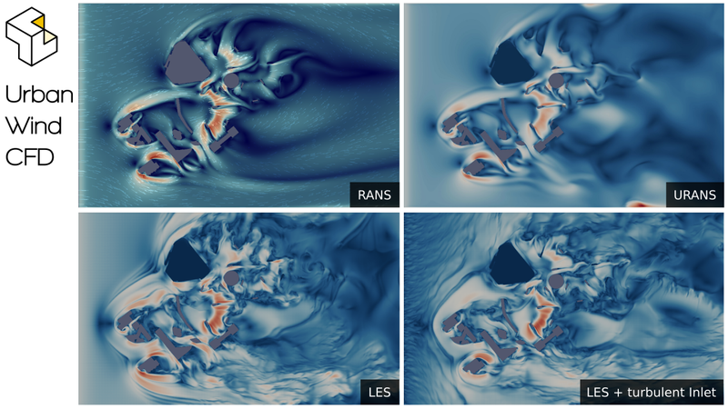
Before we jump into more detailed explanations of the respective methods, take a minute to look at this short video showing a direct comparison of simulations using the same geometry and - mostly - identical boundary conditions. Watching the video will give a much more tangible impression of the difference between the methods (see below for a 3D animation of the URANS and LES) and of why it is important to properly select and validate the model for urban wind simulation.

When looking at the video, keep the massive scale and video speed in mind. The simulation domain has a size of roughly 800 x 1200 x 400 m (WxDxH). To fill this volume with air, you need ~500 thousand tons of it. The video plays back at 10x speed; seen at this scale and with this speed, you really do get an impression of the amount of inert mass that moves around us with wind. We also made a 3D animation of the architecture with a streamlines visualization.

Solver overview

Simulations that describe the average wind field are called steady-state or intransient simulations. Often, such simulations will show a good representation of the actual average situation (in some cases the result can be ambiguous). Usually, such simulations are done based on a steady-state RANS model: a Reynolds-Averaged Navier-Stokes model. The computationally easiest and often most cost effective way to get a dynamic simulation is to implement the RANS model as the so called unsteady RANS or URANS model. In this model, the flow is permitted to vary over time, providing the basis for a dynamic simulation.

However, in the URANS model, too, turbulence is modeled based on certain assumptions, rather than as something that emerges naturally from the underlying Navier-Stokes equations, which makes the model very effective, but not particularly exact. To capture the transient behavior even better, so-called LES models are used. A Large Eddy Simulation will use exact solutions down to a certain length scale and will only use modeled turbulence beyond that. This approach tends to capture the transient behavior of wind better (especially on smaller scales), but needs more computational effort and is more difficult to implement (amongst other things because it depends on cell size).

DES (Detached Eddy Simulation) are methods that fall between (U)RANS and LES. Based on a specific criterion, the model switches between the two approaches. Not completely surprisingly, smoothly handling the transition between the two is the main issue here.

Beyond these, there is the DNS (Direct Numerical Simulation, in this context), which is basically a simulation based on the Navier-Stokes equations, but without any assumptions about turbulence. Unfortunately, due to its very high computational effort, this method is not practical for all but the most trivial cases.

RANS vs. URANS

As you can see in the video, the RANS simulation shows a good approximation of the average flow that develops with the URANS approach. Actually, one advantage of RANS is that, instead of waiting until the velocity front has moved through the entire geometry to see the final flow field, you get that result directly. For very large geometries and low wind speed, RANS is therefore a good method to get a first impression of the flow that will eventually ensue. Conversely, if it is important to see how the flow changes, RANS is not enough.

URANS vs. LES

The difference between URANS and LES is quite apparent from the video. What may not be so apparent are the similarities. If you look closely, you will see that URANS captures the dynamic overall flow situation quite well, but contrary to LES, does not resolve the small-scale variation of the flow. This makes URANS a good method to, for example, judge wind comfort. It will cover possible oscillating flow situations and show areas with higher wind velocities. LES will additionally show the strength and frequency of small-scale gusts, which is important for example for wind turbines which are sensitive towards these high-frequency velocity changes. To give even better results, LES may be done with special inlet conditions to introduce the natural velocity variations of real-life wind.

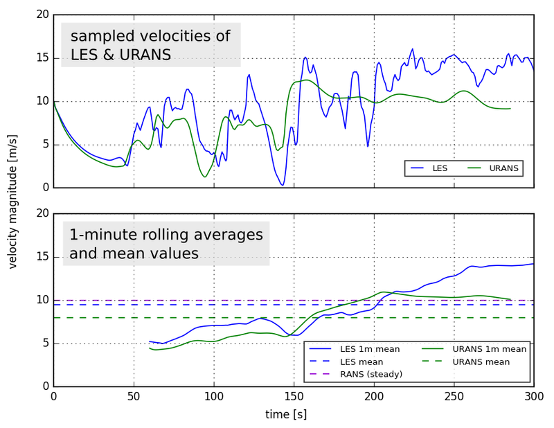
In this graph, we show the velocity over time of a single sample point in a location with high velocity changes. As the upper panel shows, the URANS simulation is a decent approximation of the LES, though higher frequency gusts are only captured by the latter (important for a wind turbine site assessment, for example). The lower panel shows the one minute rolling average and the overall mean velocities for the sample point. The mean values are all in the same range, with the LES result being quite close to the steady-state RANS simulation.

Atmospheric Boundary Layer (ABL) and (synthetic) gusts

If you look closely at the URANS and LES simulations above, you will notice that in both cases, the flow is remarkably stable around and upwind of the first buildings. In fact, there are some places that look almost exactly like they do in the steady-state simulation, with hardly any time variation at all. The reason is that the wind inlet for these simulations was set up with a simple velocity gradient to account for the Atmospheric Boundary Layer (ABL) but without any turbulence that can usually be observed in the atmosphere. This is of course a simplification versus the real case. For this reason, we use generated synthetic eddies (what pedestrians experience as gusts) in addition to the ABL velocity profile (wind velocity increases with height) to provide more natural inlet conditions for the LES solver. In some cases, we also use a combined technique: we simulate with (U)RANS first, take the velocity output from that, add synthetic eddies (gusts) and use this as input for the LES. This allows us to cover very large areas (in excess of 25 km²) to calculate an approximate wind field and use that as input for the spatially smaller, but computationally more demanding LES.

Use cases: urban planning, alpine wind parks, malls and airports

Large-scale dynamic simulations have a variety of applications for communities and architects in urban planning (from placemaking to UAV delivery), for wind energy enterprises’ in-site assessments and repowering projects, for real estate developers and even airport operations, where large man-made structures may influence conditions on the airfield. In all these cases, dynamic simulations can provide crucial planning information or may help to alleviate existing problems.

3D visualization of URANS and LES

Below, you can see a 3D visualization of the URANS, LES and LES with special inlet conditions. The playback of this video is slower than above (5x real time) and the velocities are shown in several planes and as isolines (lines of equal velocity). While the horizontal projection in the video above works fine for comparing the different approaches, the video below gives a better impression of the three-dimensionality of the flow.

Whatever your specific case looks like, we probably have the particular solver in our repertoire that gives you the best information with the least amount of associated cost. Drop us a line and let’s talk! We are happy to take a look at your project. The first consultation is always free!

Published: 08 June 2018